• Display tools
  • Display aligned windows: AlignWindowHorV.s
  • ROI (rect) synchronized on two images: SyncRectOn2Img.s
  • Display 3D-slices as film roll: FilmRoll.s
  • Display in pseudo color: PseudoColorBlueWhiteRed.s
  • Display two images with same LUT: SameDisplaySetting.s
• Calibration tools
  • Copy calibration: snippet below
  • Coply image-tag: snippet below
  • Save image-tag as .gtg file: snippet below
  • Save global-tag as .gtg file: snippet below
  • Diffraction centering using ROI: DiffOriginByROI.s
  • Diffraction centering using Numpad: DiffOriginByNumpad.s
• Analysis tools
  • Offcentered rotational averaging: OffCentRotAve.s
  • Conversion 1/nm to mrad: nmInvTomrad.s
  • Cosine and diffracion similarities of stacked diffractions: CosDifSimilarities.s
  • NMF using Scikit-Learn on DM: primitiveNMFonDM.py
• Experimental tools (in prep)
  • Peak tracker: PeakTracker.s
  • Multiple STEM imaging: (in prep)
  • Through-focus TEM imaging: (in prep)
• Disclaimer

Display tools

Display aligned windows: AlignWindowHorV.s

２つのWindowを縦あるいは横に並べて表示。
Display two windows side by side vertically or horizontally.

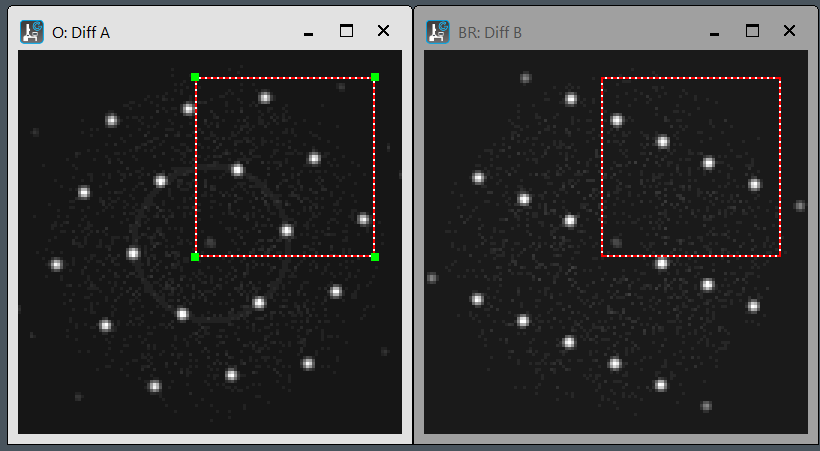
ROI (rect) synchronized on two images: SyncRectOn2Img.s

２つの画像に同じROI(Rectangle)を同期するように設定。1番上の画像のROIを参照にして2番目の画像にROIを配置・同期。同じ場所を切り出したい場合などに使用。
Set the synchronized ROIs (rectangle) on the frontmost two images. Use the ROI on the top image as a reference to place and synchronize the ROI on the second image. It might be useful when you want to crop the same area.

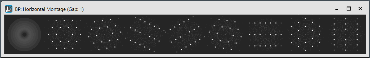
Display 3D-slices as film roll: FilmRoll.s

3Dスタック画像を、縦あるいは横につなげて２次元表示。並べて観察したい場合、同じLUTで観察したい場合に。
Display 3D images vertically or horizontally as a 2D film roll. For cases where you want to view them side by side or observe them using the same LUT.

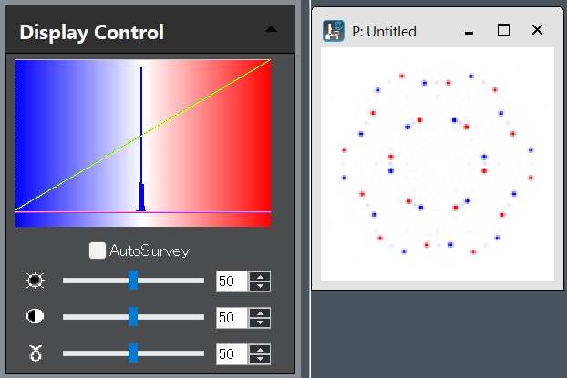
Display in pseudo color: PseudoColorBlueWhiteRed.s

決まった強度範囲を青－白－赤の疑似カラーで表示。
Display a specified intensity range using blue-white-red pseudo-colors.

Display two images with same LUT: SameDisplaySetting.s

一番上の画像と同じ表示条件(表示強度範囲やカラーテーブル)で、２番目の画像を表示。
Display the second image using the same display conditions (display intensity range and color table) as the top image.

Calibration tools

Copy calibration: snippet below

// Copy Image>Calibration from image to image
image imgfrom, imgto
if(!GetTwoLabeledImagesWithPrompt("Select 'Source' and 'Target' images","Copy ALL Tags.", "from", imgfrom, "to", imgto)) exit(0)
ImageCopyCalibrationFrom(imgto, imgfrom)

Coply image-tag: snippet below

// Copy Image>Tags from image to image  
image imgfrom, imgto  
if(!GetTwoLabeledImagesWithPrompt("Select 'Source' and 'Target' images","Copy Image-Tags.", "from", imgfrom, "to", imgto)) exit(0)  
TagGroup SourceTags =ImageGetTagGroup(imgfrom)  
TagGroup TargetTags =ImageGetTagGroup(imgto)
TagGroupCopyTagsFrom(TargetTags, SourceTags)  

Save image-tag as .gtg file: snippet below

// See and Save ImageTag as .gtg file
Image img := GetFrontImage()
TagGroup Itg = img.ImageGetTagGroup()
Itg.TagGroupOpenBrowserWindow( GetName(img) + "_tg", 0 ) 
if(!OkCancelDialog("Save this image tag?")) exit(0)
string path
SaveAsDialog("Save this global tags as .gtg", path, path)
TagGroupSaveToFile(Itg,path)

Save global-tag as .gtg file: snippet below

// How to See and Save Global Tag as .gtg
TagGroup Gtg =GetPersistentTagGroup( )
Gtg.TagGroupOpenBrowserWindow( "Global tags", 0 )
if(!OkCancelDialog("Save global tag?")) exit(0)
string path
if(!SaveAsDialog("Save this global tags as .gtg", path, path)) exit(0)
TagGroupSaveToFile(Gtg,path)

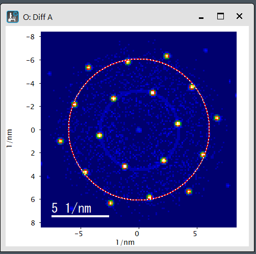
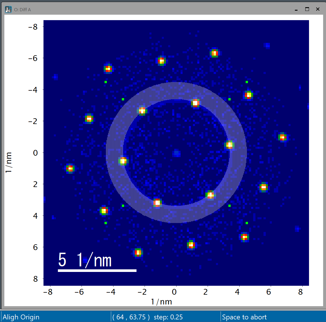
Diffraction centering using ROI: DiffOriginByROI.s

このscriptを使うと、ROIで回折図形の中心にpoint(+)をおいたり、あるいは同じ面間隔の回折スポットを通るようにoval(〇)を描き、原点を決めることができます。
Using this script, you can place a point (+) at the center of the diffraction pattern within the ROI, or draw an oval (○) passing through diffraction spots with the same plane spacing to define the origin.

Diffraction centering using Numpad: DiffOriginByNumpad.s

Originを少しずつ動かして確認。数字の4(左)、6(右)、8(上)、2(下)で、動くステップは+(2倍)、-(半分)、/で元のステップ値に戻し、スペースバーで決定。例えば、ROIのBand Pass tool(ドーナッツのようなマーク)をおいておくと、原点を中心とする円を描きますのでそれを見ながらスポット位置の調整が可能。
Gradually move the origin to verify. For the numbers 4 (left), 6 (right), 8 (up), and 2 (down), the movement step is +(doubled), -(halved), or / to return to the original step value; press the spacebar to confirm. For example, if you place the ROI Band Pass tool (the doughnut-like icon), it draws a circle centered on the origin, allowing you to adjust the spot position while viewing it.

Analysis tools

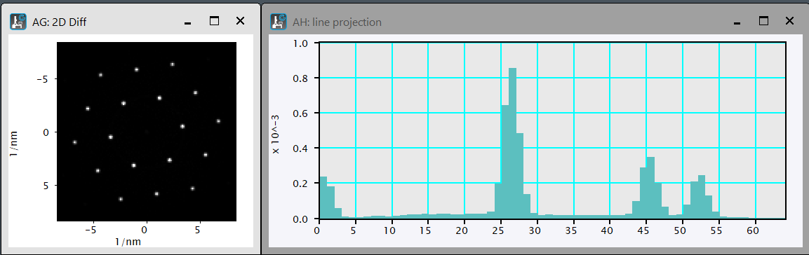
Offcentered rotational averaging: OffCentRotAve.s

2次元画像を原点座標を中心に回転平均した1次元データを表示します。
Rotatial averaged 1D of 2D image around the origin coordinates.

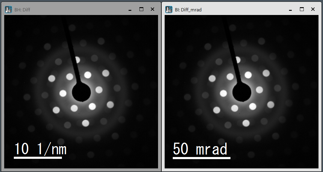
Conversion 1/nm to mrad: nmInvTomrad.s

通常、画像取得装置では、面間隔[nm]への変換が簡単になるように、回折図形は[1/nm]でキャリブレーションされています。一方、収束角などの実験条件は多くの場合には角度[mrad]で指定されています。しばしば実験条件を[mrad]で確認したいためこのscriptを作りました。加速電圧(V)によって波長(λ)が変わるため、散乱角2θと面間隔の逆数(1/d)との関係も変わります(2θ＝λ(V)/d)。そのため変換には加速電圧情報が必要です。通常の実験データでは加速電圧はimage tag（”Microscope Info:Voltage”）に保存されています。 次のscriptでは、[1/nm]を[mrad]に変換し、ファイル名に_mradをつけます(生データを間違って上書きしないようにするため)。加速電圧のtag情報が無い場合には、GetNumber()で入力を求めます。
Diffraction patterns are often calibrated in [1/nm] to simplify conversion to lattice spacing [nm]. Meanwhile, experimental conditions are often specified in angular units [mrad]. This script converts [1/nm] to [mrad]. Since the wavelength (λ) changes with the accelerating voltage (V), the relationship between the scattering angle 2θ and the reciprocal of the lattice spacing (1/d) also changes (2θ = λ(V)/d). Therefore, the accelerating voltage is required for the conversion. The accelerating voltage of each experiment is usually stored in image tag (“Microscope Info:Voltage”). The script converts [1/nm] to [mrad] and appends _mrad to the filename (to prevent accidental overwriting of raw data). If the acceleration voltage tag information is missing, it prompts for input using GetNumber().

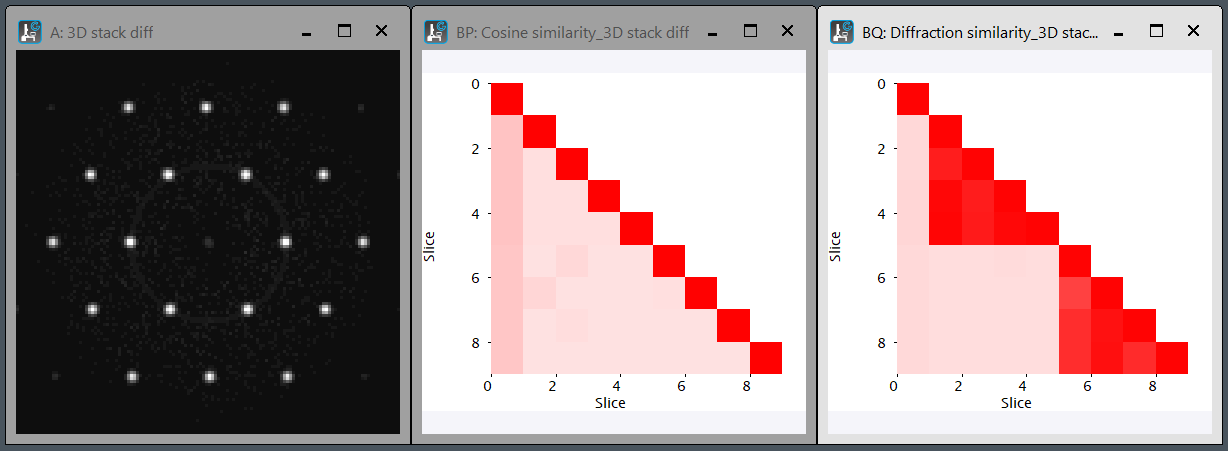
Cosine and diffracion similarities of stacked diffractions: CosDifSimilarities.s

回折図形をスタックしたデータに対して、cosine similarityとdiffraction similarityを計算し、ヒートマップを描画します。Diffraction similarityを計算するために、極座標変換も行っています。ヒートマップをscript内部で作り、-1か1までを青－灰色－赤で表現します。3Dデータ 3DStackDiffs.dm4 も参考にして下さい。
Calculate cosine similarity and diffraction similarities of 3D stacked diffraction patterns. To calculate the Diffraction Similarity, we also perform a polar coordinate transformation. Colur look-up-table, blue-gray-red is generated to cover the intensity from -1 to 1. Please refer to the link for a 3D stack of the diffraction patterns, 3DStackDiffs.dm4, for reference.

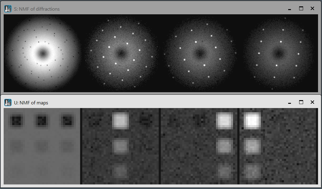
NMF using Scikit-Learn on DM: primitiveNMFonDM.py

基本的な非負値行列因子分解(nonnegative matrix factorization, NMF)を、pythonライブラリ Scikit-learnを使って、DigitalMicrograph上で実行します。DM上のpythonは標準ではScipyやscikit-learnは含まれていませんので、pipインストールする必要があります。参考となるデータSimulated4DSTEM.zipも提供します。
Primitive nonnegative matrix factorization (NMF) using Scikit-learn on DigitalMicrgraph. Python libraries (e.g., SciPy and scikit-learn) should be installed on DigitalMicrograph. The 4D-STEM data of the DigitalMicrograph format (*.dm4) can be directly processed using these libraries. The script is the Python code for primitive NMF. Note the order of the coordinates (x, y, u, v) of the DM conventional 4D-STEM data. Simulated 4D-STEM data Simulated4DSTEM.zip is also provided.

Experimental tools (in prep)

Peak tracker: PeakTracker.s

　時々刻々と変化するスペクトルやラインプロファイルに対してこのscriptを使うことにより、peakの半値幅やピーク位置のドリフト、電流[pA]、最大値などを連続的にモニターできます。EELSのzero-loss peakを主たるターゲットをして用意しましたが、プローブ電流の設定やDiffraction spotの調整などにも使えます。更新頻度やWindowの位置は、28行目のからのパラメーターで設定してください。
　By using this script on a live-view of spectra and line profiles, one can monitor full-width at half maximum, peak drift, probe current [pA], and maximums. Although I prepared primarily for zero-loss peak of EELS , it can also be used for monitoring probe current and other alignment. Please configure the update frequency and window size/position using the parameters starting on line 28.

---

そのほか、グループで利用しているscriptとしては次のようなスクリプトがあります。今後公開していく予定です。
I am planning to release the following scripts, which are used in our laboratory.

Multiple STEM imaging: (in prep)

Through-focus TEM imaging: (in prep)

Disclaimer

THE SOFTWARE IS PROVIDED “AS IS”, WITHOUT WARRANTY OF ANY KIND, EXPRESS OR IMPLIED, INCLUDING BUT NOT LIMITED TO THE WARRANTIES OF MERCHANTABILITY, FITNESS FOR A PARTICULAR PURPOSE AND NONINFRINGEMENT. IN NO EVENT SHALL THE AUTHORS OR COPYRIGHT HOLDERS BE LIABLE FOR ANY CLAIM, DAMAGES OR OTHER LIABILITY, WHETHER IN AN ACTION OF CONTRACT, TORT OR OTHERWISE, ARISING FROM, OUT OF OR IN CONNECTION WITH THE SOFTWARE OR THE USE OR OTHER DEALINGS IN THE SOFTWARE.